
Robot Plant Agents
A virtual reconfigurable garden studying plant behavior
Group Research Project for Professor Kirstin H. Petersen’s Bio Inspired Coordination of Multi Agent Systems course, Spring 2019, Cornell University
Joshua Diaz (B.S.,2019, Electrical & Computer Engineering), Elena Sabinson, (PhD. expected 2023 , Design + Environmental Analysis), Jeremy Storey (M.Eng, 2019, Electrical & Computer Engineering) and Erika Yu (M.Eng, 2019, Electrical & Computer Engineering)
This project develops a model for a virtual garden with two species of edible plants. The behavior of the plants is derived from experiments with a real-world model; the conditions of the physical experiment are reflected in the simulation. The virtual model also assumes that plants are attached to mobile robotic platforms so that they can self-organize in an optimal position to receive resources. We adopt a multi-agent system with robot-plant-agent (RPA) hybrids that are capable of sensing light and water, and rearranging their position in the environment.
This approach addresses some limitations of industrial farming where crops have limited diversity and placement, as reconfigurable gardens may increase plant survivability and yield. By enabling RPAs to change placement based on their individual needs, the robot-assisted mobility increases the system’s autonomy so that less human interference is needed. Mobile RPAs can be used in environments with no pre-existing infrastructure and in terrain that is difficult to navigate. This virtual model can contribute meaningful insights that may assist in the establishment of autonomous farming systems on other celestial bodies, such as Mars or the Moon. This research topic has the potential to produce novel contributions in the field of bio-inspired algorithms, agricultural applications, and provide a deeper understanding of plant behavior in the natural environment.
Real World Plant Experiments

Observations were recorded daily, including the day the seed first sprouted above the soil level and mortality.
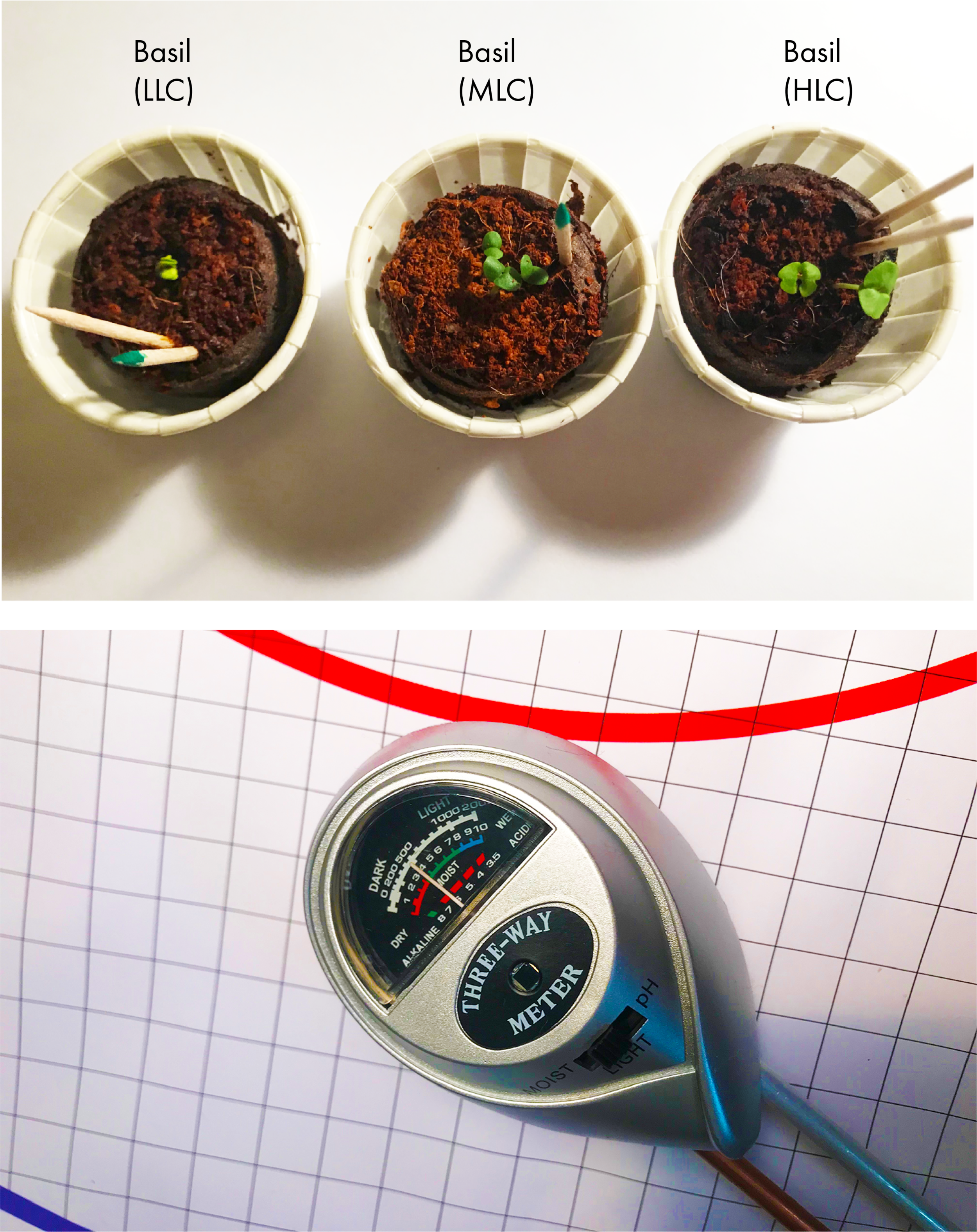
Two edible plant species were selected for the real-world plant experiment, a high light plant (HLP) and a low light plant (LLP). Beets were selected because they thrive in low-light conditions (LLC); Basil requires high light conditions (HLC) and emits high levels of VOCs. A total of 24 plants were included in the experiment, with 12 of each plant type. Seeds of both plant types were planted in starter seed pellets, which help to ensure that all plants were deposited in soil with comparable density and nutritional content.
The model space was comprised of two concentric circles printed on paper board to delineate High Light Conditions from Low Light Conditions.
The interior of the circles was filled with a half inch grid to assist in determining and tracking the plants’ location on the board. A 60 W grow light bulb was positioned to produce a gradient of light, with the highest lighting conditions centered on the board. Four lighting conditions were recorded using a light meter, and defined by the number of lumens reaching the board in a given location: low-light (LL;0-300 lm), medium-low-light (MLL; 300-600 lm), medium-high-light (MHL; 600-900 lm), and high-light (HL; 900-2000 lm). Two water conditions were tested, a subset of the plants in each lighting condition were assigned to receive water every day or every other day. Each plant was marked with its plant type and assigned light and water conditions. Plants that rotated between two lighting conditions were moved every day; both locations were marked on the board so that they were placed in the same spot at each rotation.

Seventeen of the plants in the experiment (n = 24), were still alive at completion; eleven of the HLP (n =12) and six of the LLP (n =12). The mean height of the HLP (x = 4.24 in) was substantially lower than the LLP (x = 0.793 in). This was caused by natural differences in the growth rate between the two plant species.

Observational data from the plant experiment was essential in the formation of the virtual garden, as it ensured that the behaviors modeled in the simulation were grounded in accurate representations of plant behavior within a similar environment.
Both plant types thrived in the rotating light conditions, providing evidence that reconfigurable gardens may help to increase crop yield and survivability. Furthermore, since the HLPs grew tallest in the HLC, and LLPs also grew quite tall in the LLC, second only to the rotating condition, it is reasonable to assume that plants will benefit when rearranging themselves into a position with the optimal light quality.
Both of these observations were translated into algorithmic behavior of the RPAs that move through different light conditions, and seek a place in optimal light according to plant type.
Another important observation was the importance of suitable water conditions. Too much water in LLC conditions led to mold in the soil causing the plant to die. Too little water in the HLC also killed the plants as they quickly became dehydrated without constant moisture.
This was incorporated into the model through the RPA water resource behavior, whereby agents seek water but cannot stay in the position to receive water for too long. In this way, plants obtain the resource, but quickly return to their optimal light conditions in order to prevent mold from forming and drowning the plants.

Virtual Model & Simulation

Our measure of success for this model is the number of plants that are able to survive in the system, thus, a method of determining how the plants would die is required. Our algorithm classifies as a stochastic, abiotic, resource based algorithm since the plants solely die with increased likelihood if they have lower quantities of resources.
Plants have three internal quantities that are checked at every time step to see if they die or not: Health, Sun_Health, and Water_Health. Sun_Health and Water_Health are both numbers in [ 0 , 70 ], while Health is a number in [ 0 , 140 ]. Sun_Health and Water_Health are defined by the history of the simulation, while Health is strictly the summation of Sun_Health and Water_Health. Each agent generates a random number at every timestep between 0 and 100. If this roll is greater than the current Health of the agent, that agent dies. Otherwise they can continue living in the system. In short, the higher an agent’s health is, the lower their chance of dying. The Sun_Health and Water_Health have upper bounds greater than 50 to give agents a benefit to absorbing a larger amount of a resource than required. For example, a plant that has been watered a significant amount recently does not need more water in the near future.Once an agent dies, it is ignored by the other agents currently in the system and cannot move or interact. For simplicity’s sake, dead agents only exist graphically on the simulation screen.
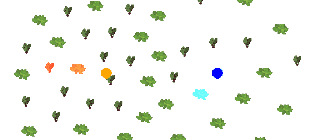
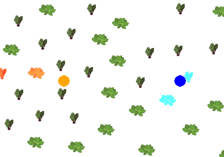
Light & Water Resources

Water is a point source with a binary, fixed health gain or decrement.
Only agents within a certain radius of the water source’s center, will increase their health by 2. Agents that are outside this circle will lose 0.25 health. The amount of health gained/lost was chosen based on qualitative observations of our simulation runs so that the agents lived long enough to interact with other agents or reach their resource goal, with the ultimate goal of tuning the resource behavior from observations from real life plants.
Light resource contributes to health following a continuous function.
Each plant type is specified an optimal sun value corresponding to the distance away from the light source where an agent gains the most health. As the agent moves farther away from its optimal value, the health gained will decrease, approaching a constant negative value. Movements toward and away from the light source are treated equivalently. The equation used to determine the amount of Sun_Health gained is: Δhealth =(p+q)e-(b*dist2)-q, where p is the maximum amount of health gained at an agent’s optimal sun value, b is an exponential decay constant, dist is the distance of an agent from its optimal value, and q is the maximum health lost when an agent is far away from the optimal. P and q were chosen to be 2 and 0.25, respectively, to match the values used to change the agent’s water health.
Light and Water Attractors. Plant agents seek optimal resources to maintain health based on plant type.
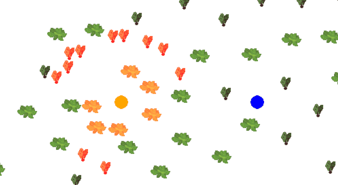
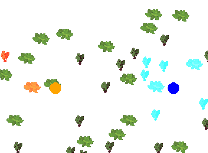
VOC signalling

A repulsive force used to direct plant motion, inspired by plant communication through airbone VOC signals.
An artificial signalling model was developed as a representation of plant communication through airborne signaling systems used by plants in response to environmental stimuli. Volatile organic compounds (VOCs) are chemical emissions plants use to relay information about their physiological states and environmental conditions. It also produces allelopathic effects, whereby a plant dissuades competing plants from growing in a nearby location.
VOCs operate as a mediator between plants and other organisms. A bio-inspired algorithm that explores this plant behavior in a virtual garden may provide insights into these biological signaling networks.
In the model, emission of VOCs is the only method, other than direct collision, by which plant agents can communicate. It is modeled as a repulsive force between plant agents whose effect on a given plant, a, is the weighted vector sum of VOC forces between every other agent and itself. This sum is then normalized to a velocity parameter, v, which is the max velocity that the agent can physically move (and that it moves toward throughout the entire simulation). The magnitude of the VOC repulsion felt on an agent a by just one other agent b is proportional to plant b’s stress parameter scaled exponentially by the distance between the two and the stress emittance parameter. The force is along the vector between a and b, pointing towards a. The total effect on a’s velocity by all agents is thus:

Stress is accumulated purely by a plant’s inability to retrieve whichever resource it is actively seeking. The value of stress increases at the same rate that a plant’s health decreases.
For instance, should a plant be in need of water, but unable to reach the resource, its health reduces by 0.25. At the same time, its stress is increased by 0.25, pushing agents away. Emittance is set as an intrinsic property of the plant, and is initialized at plant creation.
Model with no VOC signalling led to deadlocks
Model with VOC collision behavior implemented